ATNIX: Australian Twitter News Index, March 2015

Compared to the excitement of January and February, March 2015 has turned out to be a comparatively quiet month in Australian public life, even in spite of the New South Wales state election campaign which culminated in the re-election of Mike Baird’s Coalition government on 28 March. The immediate heat has dissipated from the leadership debate around PM Tony Abbott: contenders Malcolm Turnbull and Julie Bishop are resorting to playing the long game and as any potential new leadership challenge looks increasingly unlikely to happen before the May budget.

For the purposes of our Australian Twitter News Index (ATNIX), which tracks the sharing of links to Australian news and opinion sites on Twitter, this period of relative calm manifests in comparatively stable, regular link sharing patterns. ABC News and the Sydney Morning Herald continue to track neck-and-neck with some 315,000 to 320,000 links shared throughout the month, and are firmly established as Twitter news market leaders in Australia, with third-placed The Age reaching only some 135,000 tweets over the same period.

The major point of heightened activity during the month occurs in the week of 16 March, especially for ABC News, as the full aftermath of tropical cyclones Nathan (off far north Queensland), Olwyn (northwestern Australia), and – most devastatingly – Pam (which caused severe destruction in Vanuatu) became known. A report that several elderly indigenous residents in Carnarvon were denied access to a cyclone shelter ahead of Olwyn’s arrival was especially widely retweeted. Meanwhile, a particularly spectacular Aurora Australis event which was visible even from the mainland generated additional shares for the ABC.

image

Meanwhile, major political stories fail to emerge beyond general day-to-day sharing. The Australian records a brief spike in shares on 2 March with an article suggesting that a major ally of Indonesian President Joko Widodo had come out against the death penalty for Bali Nine drug smugglers Myuran Sukumaran and Andrew Chan, and PM Tony Abbott’s swiftly withdrawn comparison of Bill Shorten with Joseph Goebbels in parliament causes a brief flurry of outrage on 19 and 20 March, but there is little sustained engagement with either of these stories, beyond average levels.

And finally, the comparatively uneventful end to the NSW election campaign (at least by contrast to the surprising outcome of the Queensland poll, one month earlier) similarly fails to significantly affect the sharing of links to Australian news and opinion sites – indeed, 28 and 29 March are the days which see the fewest links to the Sydney Morning Herald shared during March, even compared to the already lower weekend averages for the paper.

image

Such a lack of sharing does not represent a lack of interest in the results of the New South Wales election, however. Turning to our Experian Hitwise data, which show the total number of user visits to the leading Australian news and opinion sites, we can see that the Sydney Morning Herald and – especially – ABC News record comparatively strong results on 28 and 29 March; with almost 770,000 visits to its site, ABC News in particular receives as many visitors on the Sunday as it usually does on weekdays. This points strongly to the ABC’s continuing role as the nation’s premier source of information on election results – similar to the patterns we observed in the previous Queensland election.

However, especially in the absence of any major election surprises, it is also evident that Twitter and (presumably) other social media users did not feel the need to specifically share the NSW election results with their followers and friends: the elevated levels of access to the ABC and other news sites on and after election day did not result in significant additional shares. Had there been any unforeseen developments, the picture would likely have been very different.

Standard background information: ATNIX is based on tracking all tweets which contain links pointing to the URLs of a large selection of leading Australian news and opinion sites (even if those links have been shortened at some point). Datasets for those sites which cover more than just news and opinion (abc.net.au, sbs.com.au, ninemsn.com.au) are filtered to exclude the non-news sections of those sites (e.g. abc.net.au/tv, catchup.ninemsn.com.au). Data on Australian Internet users’ news browsing patterns are provided courtesy of Experian Marketing Services Australia. This research is supported by the ARC Future Fellowship project “Understanding Intermedia Information Flows in the Australian Online Public Sphere”.

Metrics for Analysing Twitter Communities, Using TCAT and Tableau

This post builds on the new approach to transforming Twitter datasets generated by the TCAT tracking tool for analysis in Tableau which I’ve introduced in my recent posts. Often, we will be interested in exploring the structure of Twitter communities as they form around given hashtags or keywords – for instance to examine whether they really act as communities in a narrow sense, or are rather merely groups or publics who are in some way connected to the hashtag, but barely aware of each other’s presence.

In the past, we’ve used one of our Gawk scripts, metrify.awk, to generate a range of metrics which provided detailed information on the dynamics of a dataset over time, across individual users, and across different groups of accounts as defined by their level of activity; I explained that process in a multi-part post in 2012 (1, 2, 3, 4, and follow-up). With the move from yourTwapperkeeper and Excel to TCAT and Tableau, most of this analysis can now be done directly within Tableau itself, directly from the source TCAT dataset and the additional helper datasets which our TCAT-Process scripts generate. What’s still missing from the mix is a method for exploring the contribution of the different groups of accounts, though – this post outlines the steps for generating these metrics from within Tableau itself.

Introducing Percentile Groups

It’s well established that the distribution of activity levels across a given group of social media accounts will often follow a ‘long tail’ distribution: a very small number of accounts are very heavy contributors to a hashtag or a discussion, while a large number of others are contributing only very occasionally. The exact balance between these groups, and the exact nature of their respective contributions, can tell us a great deal about the dynamics of the overall Twitter public gathered around the shared hashtag or theme – the lead users may contribute in different ways from the least active users, for example by including more URLs in their tweets, or by taking a more discursive approach that features more @replies than retweets. We’ve used such observations very effectively in the past to distinguish between different types of hashtag events, and to pinpoint useful areas for further close reading of tweets.

What’s often used in this context is a 1/9/90 division between participants: ordered by their number of contributions to the conversation, the top 1% of accounts are identified as lead users; the next 9% as highly active users; and the remaining 90% as least active users. Other divisions are also possible, of course; what is most appropriate will depend on the specific dataset at hand, and on the research questions asked of it. For the purposes of this post, we’ll continue with the 1/9/90 division of accounts into three percentile groups.

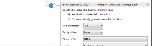
Happily, it is fairly straightforward to create these percentile groups in Tableau. In the following discussion, I’m building on the processes outlined in my previous posts: so, we’ve already downloaded a full dataset export from TCAT (in my example, tweets about the attempted party leadership challenge to Australian Prime Minister Tony Abbott, using the #libspill hashtag and a number of related hashtags and keywords), and we’ve processed this dataset using the TCAT-Process scripts package I’ve made available here. We’ve also loaded and combined the resulting datasets in Tableau.

Now, the first new step is to create a new calculated field called ‘Percentile Ranking’ in Tableau, using the following formula:

RANK_PERCENTILE(COUNTD([Id]))

As usual, we are using COUNTD(Id) as the most reliable count of unique tweets; in a given list of items in Tableau, the RANK_PERCENTILE() formula then uses this count of tweets to calculate which percentile in the list a specific item occupies. The result will be a value between 0 (lowest percentile, 0%) and 1 (highest percentile, 100%).

In Tableau, we can now graph CNTD(Id) against From User Name, order the list by CNTD(Id), and add Percentile Ranking as a label; this generates an ordered list of participant accounts and shows their percentile ranking:

image

By this ranking, accounts with a Percentile Ranking greater than 0.99 are in the top 1% of lead users; accounts with a ranking between 0.9 and 0.99 are in the next 9% of highly active users; and the remainder of accounts with a ranking below 0.9 are in the bottom 90% of least active users.

However, in our further analysis we cannot use the Percentile Ranking field directly, as it is always freshly calculated depending on what fields are graphed against each other; we therefore have to persistently allocate accounts to the three groups we’ve defined. This is where Tableau gets uncharacteristically cumbersome for a moment:

  1. First, add Percentile Ranking to Filters, and filter for accounts with a ranking of at least 0.99:
    image
  2. Next, click anywhere into the white space in the graph, and press CTRL-A to select all visible rows. Mouse over one of the rows, and click the paperclip icon to create a group:
    image
  3. The new group will appear in the Dimensions sidebar, as “From User Name (group)” – rename it to something more meaningful, such as “LU” (for Lead Users).
  4. Remove LU from the Color field, where Tableau has placed it automatically.
  5. Change the Percentile Ranking filter to a range of values between 0.9 and 0.99, and repeat the previous steps – call this new group “HA” (for Highly Active).
  6. We now have two separate groups of accounts – LU and HA – and at least implicitly also a third group of accounts who belong to neither LU nor HA: these are our 90% of least active users. The final step is to combine these individual groups into one unified categorisation scheme which we can use in our further analysis: in the Dimensions sidebar, shift-click on the two groups to select them, right-click on one of them, and select Combine Fields – this finally creates a new combined field that permanently assigns each user to one of the three groups:
    image
  7. Finally, let’s rename the new combined field “LU & HA” to “Sender Groups”.

(The overall process will remain the same for different percentile cutoffs, of course, and is even easier if you make only a simple distinction between a lead user group and the remainder of the userbase – for a 20/80 split, for example, simply create one group for accounts ranked above .8. However, finer gradations between multiple subgroups usually generate more useful analysis.)

Analysing the Groups’ Contributions

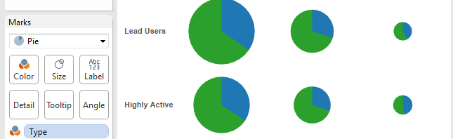
Having created these groupings, we can now begin to use them in our analysis. First, we should determine how many accounts there are in each of our groups, by showing the count of unique user names – i.e. CNTD(From User Name) – for each of the groups (note that I have also added a Grant Total row by selecting Analysis > Totals > Show Column Grand Totals):

image

By default, Tableau names the groups after the combination of selection criteria that the combined Sender Groups field was constructed from – but from the membership size of the groups listed above we know that the smallest group (the first row in the image above) must be the 1% of lead users, the second the 9% of highly active users, and the third the remainder of the 90% least active users. Right-clicking on each field and selecting “Edit Alias…” allows us to rename these fields to something more user-friendly.

It is also notable that while my dataset contains a total of 134,518 unique user names, the lead user group is made up of 1,347 accounts, and the two top groups together number 14,396 accounts in total – more than the 1% or (combined) 10% of 134,518 that they should contain. This is not an error, but simply a sign that Tableau does not play favourites: if there are multiple accounts at the boundary between two groups which equally fulfil the requirements for belonging to the higher-ranked group, Tableau will include them all, rather than arbitrarily sending some of them to the lower group in order not to expand the higher percentile group beyond the top 1% or 10%. In my sample dataset, for example, the cutoff for belonging to the lead user group was a total of 43 tweets sent, and multiple accounts had reached exactly that number.

Next, we might want to explore the number and types of tweets sent by each group – so here, I’ve graphed Sender Groups against CNTD(Id), and coloured by Type (again with an added Grand Total column). What becomes evident in my sample is that the 1,347 lead users contributed more tweets than each of the other two groups, and that they were especially active in sending @mentions and retweets:

image

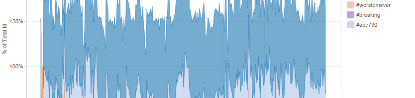
Replacing Type with Hashtag as the field determining colour, we can also determine highly divergent hashtagging practices – the lead users almost always included a hashtag, while almost two thirds of the tweets posted by the least active users did not contain hashtags (note again that the tweet numbers are increased beyond the previous graph here, and the percentages add up to more than 100%, because tweets can contain two or more hashtags). Incidentally, I’ve displayed the percentages by adding CNTD(Id) to Label and calculating its value as a percentage of total, using Table (Down) as the calculating method:

image

Many further permutations of these analyses are also possible, of course – we might explore, for example, whether there are differences in the URLs each group are sharing (are they using distinctly different domains as their sources of information?), or whether they are tweeting from notably different devices (as indicated by the Source field).

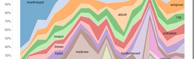
Further, we can also examine the contributions by these groups over time:

image

In my example, this shows that the lead users are responsible for a volume of tweets that usually closely matches that contributed by the (much larger) group of highly active users, while the least active users are less engaged during peak times, but make up for this by maintaining greater levels of activity outside of peak periods. This could also indicate that the least active group contains a range of users whose tweets showing up in our dataset as false positives (e.g. because they use the term ‘spill’ in non-#libspill-related contexts), which could be a good argument for excluding this group from the analysis altogether.

Using Percentile Groups Elsewhere

While this post has focussed on defining groups of accounts based on their active contributions to a dataset (i.e. the number of tweets they posted), the same approach can also be used for other distributions where grouping may be useful. For example, we might instead list the accounts being @mentioned (based on the To User field which the TCAT-Process scripts generate – not the unreliable To User Name field which the Twitter API itself provides) against the number of tweets mentioning them (via CNTD(Id)), and again calculate their percentile ranking. In fact, we can use the Percentile Ranking field we defined at the start of this post – it performs a new calculation for any list of items it is being applied to:

image

We should exclude “Null” from this list (which collects all the tweets which did not @mention or retweet another user), and can then again define a number of percentile groups following the process outlined above. For my sample dataset, this results in a group of 454 “Most Visible” accounts (the 1% of accounts who received the most @mentions and retweets), 4,596 “Highly Visible” accounts (the next 9%), and 40,272 “Least Visible” accounts (the remaining 90%). Note here, though, that by default Least Visible will contain the “Null” recipient (as Least Visible is simply a collection of all recipients that are not included in the other two groups), so we will need to manually filter out this recipient from all further analysis.

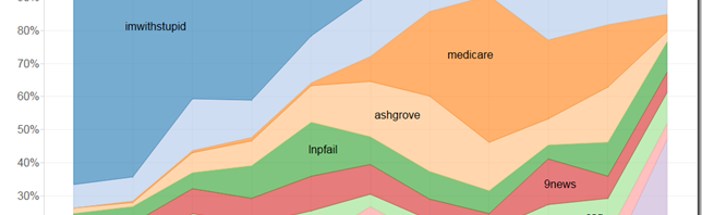
I’ve combined these groups into a Receiver Groups field, which we can now also use for some interesting analysis. First, for example, as expected the most visible accounts command the majority of @mentions and retweets:

image

Second, they are also especially popular with the most active participants in the discussion. Note especially how the least visible accounts are mainly mentioned by the least active participants – it seems that there are several separate discussion circles here:

image

And finally, turning the interactions between the various sender and receiver groups into a matrix and adding some further Tableau functionality into the mix, here’s a nice graph to end on. This shows the volume of activity from each sender to each receiver group, and breaks it down into @mentions and retweets:

image

Again, similar rankings can of course also be created for many of the other fields in our dataset – for example for the most frequently shared URLs (at the domain level, or for each fully qualified URL), the most prominent hashtags, even the most widely used tweeting platforms. Given the approaches I’ve outlined here, I hope these will be relatively easy to calculate now.

ATNIX: Australian Twitter News Index, February 2015

February 2015 has been a tumultuous month in Australian news, not least because of the continuing leadership debate (and defeated spill motion) in the federal Liberal Party following the LNP’s unexpected defeat in the Queensland state election on 31 January. As expected, these and other events also affect the patterns observed in our Australian Twitter News Index (ATNIX) and in the overall Australian online news readership patterns tracked by Experian Hitwise.

That said, the unsuccessful motion for a leadership spill on 9 February fails to generate any truly exceptional spikes in the patterns of newssharing on Twitter: we can identify some slightly elevated levels of activity around a number of news sites (chiefly, ABC News, the Sydney Morning Herald, and news.com.au), but for most sites that Monday does not even constitute their most active day of the week, let alone the month.

A likely reason for this is the blanket media coverage of Liberal leadership speculation since the Queensland state election (or even since the Australia Day news of a knighthood for Prince Philip). The Liberal spill motion was nowhere near as unexpected as the first Rudd/Gillard spill, for example – and as we have seen time and again, Twitter users are less likely to share news items when they can reasonably assume that these are widely known already.

(Abbott loyalists might also want to construe this lack of significant additional activity as an indication that Australians have no interest in all of these “Canberra insider” machinations – but that argument is undermined by the fact that we do see a very substantial amount of day-to-day sharing of articles that discuss the Abbott government and its troubles. It’s just that on 9 February there was no significantly further elevated level of sharing than on other days.)

image

This view is also supported by the fact that a number of the more dramatic spikes in sharing activity are directly related to continuing controversies over Abbott’s leadership and government policy: in other words, in sharing links to news articles Twitter users focussed more on the underlying troubles than on the spill motion which resulted from them.

One of the most surprising boosts from such activity is received by The Australian, which – partly due to its paywall – usually struggles to gain more than 2,000 Twitter shares per day: it is linked to in 4,900 tweets on 21 February, largely as a result of its coordinated attack on Abbott that Saturday, consisting of stories about Abbott’s supposed idea of launching a unilateral military intervention in Iraq, about his subsequent denial of such rumours, and about the extent of his chief of staff Peta Credlin’s power over government decisions.

Similarly, SBS draws on its growing stable of news satirists to record a spike well above average on 4 February, with a comedy piece reporting that Julia Gillard had been rushed to hospital with an acute case of Schadenfreude. Meanwhile, The Age gains particular prominence on 26 February with its coverage of the government attacks on Gillian Triggs and the Human Rights Commission, and opinion articles reflecting on the broader implications for evidence-based policy-making and for the status of women in political leadership roles.

Amidst such domestic controversies, other news stories remain somewhat less prominent. The increasing desperation over the impending executions of convicted Australian drug smugglers Andrew Chan and Myuran Sukumaran in Indonesia is manifested in only two widely shared articles: a Herald-Sun story about Indonesian President Joko Widodo’s resistance to calls for clemency on 12 February, and The Age’s coverage of protests and boycotts against Indonesia on 16 February. It is likely that we will see more such articles being shared as the legal and diplomatic efforts to avert the death penalty continue in March, however.

As always, Experian Hitwise data on the total visits to Australian news sites during February paints a somewhat different picture, compared to our ATNIX data on what articles are eventually shared on Twitter. Here, the Liberal leadership spill on 9 February results in small but pronounced increases in visits for most leading news sites – news.com.au, Sydney Morning Herald, nineMSN, The Age, and ABC News all receive clear boosts to their numbers.

image

More notable, however, is the substantial spike in visits to the Courier-Mail site on the following day, which is almost certainly related to the final stages of the transition of government in the state, as signalled by Labor leader Annastacia Palaszczuk’s visit to the Queensland governor that afternoon. A simultaneous spike in visits to the Herald-Sun site does not have any similarly obvious explanation.

Overall, however, what is more obvious here is the relative stability of overall trends – there are few major spikes in activity, suggesting that following the holidays readers have now settled back into their daily routines of reading news online. This is also reflected in the volume of total visits across the sites, which is almost identical to last month’s patterns – news.com.au, Sydney Morning Herald, and Daily Mail Australia retain their overall leadership positions, and their gaps from each other.

The only significant movement is amongst the opinion sites: The New Daily’s strong run over recent months is fading, and it falls further behind The Conversation (but remains a clear second); New Matilda surpasses The Morning Bulletin to claim fourth place on the leaderboard; and Independent Australia considerably increases its share of visits (from 86,000 in January to 400,000 this month), catching up to the leadership group.

Standard background information: ATNIX is based on tracking all tweets which contain links pointing to the URLs of a large selection of leading Australian news and opinion sites (even if those links have been shortened at some point). Datasets for those sites which cover more than just news and opinion (abc.net.au, sbs.com.au, ninemsn.com.au) are filtered to exclude the non-news sections of those sites (e.g. abc.net.au/tv, catchup.ninemsn.com.au). Data on Australian Internet users’ news browsing patterns are provided courtesy of Experian Marketing Services Australia. This research is supported by the ARC Future Fellowship project “Understanding Intermedia Information Flows in the Australian Online Public Sphere”.

Using Gawk to Prepare TCAT Data for Tableau, Part 2

In my previous post, I introduced a new set of Gawk scripts to extract a range of additional information from standard TCAT datafiles, in order to enable their use for data exploration, analysis, and visualisation in Tableau. After running the TCAT-Process scripts, we now have the following datafiles:

  • datafile.csv – the original TCAT dataset (a full export of all tweets and metadata)
  • datafile-tweettypes.tab – a helper table which for each tweet lists the users mentioned, and the type of mention (‘@mention’ or ‘retweet’) made for each user; for tweets not containing any mentions of other users, the type is set to ‘original’.
  • datafile-hashtags.tab – a helper table which for each tweet lists the hashtags it contains.
  • datafile-urlpaths.tab – a helper table which for each tweet lists the short URLs and resolved destination URLs it contains, as well as the domain and domain and first path component of the resolved URL.

In combination, these datafiles enable a very wide variety of Twitter analytics in Tableau – replacing many of the processing steps that previously required a number of additional Gawk scripts, in fact.

In this post, I’m using a TCAT dataset on the recent attempted leadership spill in the Australian federal Liberal Party to demonstrate how to use these datafiles for Twitter analysis.

Linking the TCAT-Process Outputs in Tableau

The first step in using these datafiles is to relate them to each other in Tableau. So, after opening Tableau, I’m first connecting to the original Tableau dataset. Second, I’m dragging the tweettypes.tab datafile which the TCAT-Process script has created next to my main dataset. By clicking on the circles between them, I can now choose a Left Join, and Tableau already correctly suggests joining them on the ID field:

image

This means that for every tweet ID listed in the main TCAT dataset, Tableau now also reads in the datapoints from the tweettypes.tab datafile that relate to the same tweet ID. Note that – because tweets can mention multiple other users at the same time, and can thus be both @mentions and retweets at the same time – this means that the same tweet in the main dataset can now have multiple corresponding datapoints from the tweettypes.tab file.

We’re repeating the same process with the hashtags.tab and urlpaths.tab datafiles. Again, we’re using a Left Join, and again this means that multiple datapoints from these datasets may relate to the same tweet (if it contains multiple hashtags or URLs). By clicking on the gears icon that appears when mousing over the datafile names, a number of other useful parameters can also be set:

image

Most importantly, the character set should be set to UTF-8, and (to be on the safe side) the text qualifier should be set to None – but make sure it remains set to double quotes (“) for the main TCAT dataset.

Once all of these parameters are set, we can select the Connection method (make sure you use Extract for larger datasets), and click on Go to Worksheet.

Working with TCAT Data in Tableau

Before we begin the analysis, some housekeeping and setup will be useful. Tableau tends to place the tweet ID fields in its list of Dimensions, but we’ll be wanting to use a count of unique IDs in many of our analyses, so drag the ID field from each of the four data tables into the Measures list, and select Count (Distinct) as the default aggregation:

image

Further, for some datasets there may also be a need to adjust the timestamp of tweets in order to account for different timezones. To do so, right-click on the Created At field, create a calculated field, and use Tableau’s DATEADD function to adjust the time. My #libspill data is using AEST, for example, but as Canberra (where most of the spill action took place) is on daylight savings time and thus one hour ahead of AEST, I’m creating a new AEDT time field which adds one hour to AEST:

image

By dragging AEDT into Columns, and ID into Rows (where it will automatically become a count of unique IDs – CNTD(ID)) we can now chart the overall volume of tweets. Note that we’re using CNTD(ID) rather than the non-unique CNT(ID) or simply Number of Records because by joining our helper tables with the main dataset we now have more individual records than unique tweet IDs: each second or third user mention, URL, or hashtag in a tweet adds to the total count of records, so that – in my example – the 435,000 unique tweets contained in the #libspill datasets have become almost 980,000 records in the dataset.

image

Such basic volumetrics were already possible by using only the original TCAT dataset, but what comes next is possible only because of our data preprocessing using the TCAT-Process scripts. By dragging Type or Hashtag onto the colour, for example, we’re able to see what types of tweets or which hashtags were prominent at any one point (click to enlarge):

imageimage

Similarly, the preprocessing has extracted data on the major recipients of @mentions, and the major sources of URLs being shared. Here we can use the To User and Domain fields for colour coding, and for greater clarity I’ve limited the graphs to the top 10 in each case, and filtered out any tweets which didn’t mention another user or shared a URL, respectively:

imageimage

Such graphs can also be shown as a percentage of the total for each point in time. Note that in many cases the total will add up to more than 100%, as in my example below: my dataset was gathered largely based on the #libspill and #spill hashtags, but many of the tweets contained more than one hashtag.

image

Beyond Volumetrics

Many other combinations of datapoints are also possible – too many to step through here. However, some key analytical approaches beyond basic volumetrics are particularly obvious: for example, graphing From User Name or To User against CNTD(ID) and colouring by Type, we can see not only how many public tweets individual users sent or received, but also whether these were predominantly original tweets, @replies, or retweets, or a combination of them all – and by showing the two graphs alongside each other in a single Tableau dashboard, we can also create a useful comparative graph. Here, it’s important to use our new field To User, not TCAT’s and the Twitter API’s To User Name, which is only very rarely set to any actually useful value.

image

(Note that Tableau’s sort function seems to have some trouble sorting by CNTD(ID) – you may need to make some manual adjustments…)

It may also be useful to explore in which hashtag contexts specific users are @mentioned (for the purposes of illustration, here we’ve removed the generic #libspill, #spill, and #auspol hashtags, and included only the top 10 remaining hashtags):

image

Finally, there’s plenty we can do with the resolved URLs from the tweets, too. For example, here are the most widely shared domains (including the first component of the URL path, to gain a little more insight into what the content may be), and the types of tweets they’ve been shared in. One domain sticks out as being linked to only in original tweets – a clear indication of spam:

image

If we filter for retweets only, we can see which domains were the major information sources during the event. Beyond Twitter itself (which mainly shows up because of widely shared images in tweets), we see that the sites offering liveblogs on the day (Sydney Morning Herald, The Guardian, ABC News) are especially prominent:

image

And filtering the Domain field for links to Twitter content only, we can identify the most widely shared images (disseminated mostly through retweets, as we can see), as well as a set of what we might assume to be spam links (since Twitter itself flags them as potentially unsafe, and they were disseminated largely through hundreds of original tweets):

image

Of course as always it is then possible to drill down further into the data, and identify exactly which images and articles were most salient for participants in the Twitter discussion – in Tableau, that’s as easy as viewing the underlying data for any specific graph or datapoint.

So much for a quick overview of the potential analytical approaches which the TCAT –> Gawk –> Tableau process makes possible. Perhaps a future version of TCAT might even enable a direct export of the three additional helper tables our approach has created, without a need for the additional processing work in Gawk – but for the moment, the TCAT-Process scripts package should help to further enhance existing Twitter data analytics approaches, I hope.

Using Gawk to Prepare TCAT Data for Tableau, Part 1

Much of the research we’ve presented on this site over the years has built on yourTwapperkeeper, our trusty old tool for gathering Twitter data. But yTK isn’t the most modern of platforms any more, provides only a very limited user interface, and gathers only a fraction of the full metadata payload which the Twitter API delivers alongside the tweets themselves. More recently, therefore, we’ve increasingly switched our data gathering efforts to the Twitter Capture and Analysis Toolkit (TCAT), developed by the Digital Methods Initiative at the University of Amsterdam.

TCAT has its own limitations – for one, it only utilises the Twitter streaming API, while yTK also uses the search API for backfilling tweets in case of server outages; incidentally, a side effect of this is that it’s impossible to use URLs like abc.net.au as search terms in TCAT, since the streaming API doesn’t match search terms on resolved URLs, while the search API does. (Our ATNIX project depends on this functionality, and thus continues to rely on yTK.) But overall, TCAT provides a considerably more advanced solution for gathering Twitter data these days, and so we’ve had to develop new approaches to working with the datasets it generates.

Additionally, data analytics tools have also moved on. Excel was never particularly well suited to any serious analysis, and in the past we’ve done a great deal of data preprocessing using the command-line tool Gawk before loading the results into Excel for visualisation. These days, however, the software of choice is Tableau, whose functionality is several generations ahead of what Excel has to offer and which can do on the fly much of the analysis which we’ve had to painstakingly prepare during the preprocessing stage in the past. Tableau is far from inexpensive (although it’s free for current students, and educational pricing is available), but simply has very few credible alternatives at this point.

Connecting TCAT and Tableau, via Gawk

What’s still needed, then, is a straightforward process for loading TCAT data into Tableau. TCAT already has a number of built-in export functions, but these aren’t necessarily well-suited for our purposes, given the data format Tableau prefers. What’s worse, TCAT’s full data export format has changed over time, so the structure of its outputs isn’t necessarily very standardised. In this post, then, I’m outlining a standard method for preprocessing TCAT data specifically for Tableau, and below I’m also sharing the scripts that implement this method.

We’re building here on the TCAT function which exports all tweets in a dataset, subject to the specific parameters set by the user (timeframe, text and user filters, etc.):

image

This export results in a comma-separated values (CSV) file, which can already be imported into Tableau for analysis. However, what Tableau will struggle with is to extract some of the important information which isn’t yet in the metadata: for example, which users are mentioned in a tweet, whether a tweet is a retweet or @reply, which hashtags are present in a tweet, and which URLs are being shared. The problem is that most of these elements could occur multiple times in the same tweet: for example,

Hey @friend, have you seen this? #ohno RT @news: #BREAKING: World ends. http://t.co/abcdefg

is both an @reply (or @mention, of @friend) and a retweet (of @news), and contains the two hashtags #ohno and #BREAKING. In a simple CSV which contains only one row of data for each tweet, such multiple metadata points per tweet are very difficult to represent.

This is, of course, what relational databases are useful for, and Tableau provides the functionality to link multiple data sources (even in CSV or TSV form) in much the same way as if they were tables in a database. The easiest way to do this is based on the Twitter-generated ID of each tweet, which is unique and stable. Assuming the example above has the ID 1, for example, we could generate three additional tables to document the @mentions, hashtags, and URLs contained in the tweet:

ID

@mention type

target user

ID

hashtag

ID

URL

1

@reply

friend

1

#ohno

1

http://t.co/abcdefg

1

retweet

news

1

#BREAKING

Note that the @mentions and hashtags table now each have two entries relating to the same tweet, because it’s both an @reply and a retweet, and contains two different hashtags. Additionally, it would also be useful to resolve the t.co link to its eventual destination, and perhaps to specifically extract the URL’s domain name (so later on we can examine which sites are especially important in a dataset):

ID

Domain

Long URL

URL

1

http://cnn.com

http://cnn.com/worldends

http://t.co/abcdefg

These tables can then be linked with the main TCAT datafile, which itself constitutes a large table of tweets and metadata.

Introducing the TCAT-Process Scripts

Update: I’ve made further adjustments to these scripts to make them easier to use on a Mac. Please re-download the scripts package, and note the updated instructions below.

All of this is relatively easy to do using our old friend Gawk, a programmable command-line tool which is designed to process and filter CSV/TSV-format files. Below, I’m sharing a suite of Gawk scripts that are designed to work through the following steps:

  1. Take the TCAT datafile, extract tweet IDs and texts.   –>   datafile-tweettext.tab
  2. Identify @mention types and recipients.   –>   datafile-tweettypes.tab
  3. Identify hashtags in tweets.   –>   datafile-hashtags.tab
  4. Extract and resolve URLs in tweets.   –>   datafile-urlpaths.tab
    (This – optional – last step generates a number of temporary files for error checking, which can be deleted.)

The Gawk scripts automate the entire process – once everything is installed, a single Gawk call will do all the processing. Here are the scripts, as a downloadable ZIP archive, and here’s how to install them and set everything up to go:

  • Install Gawk and cURL.
    • Windows: Gawk (complete package – except sources); cURL (Win32 or Win64 – Generic, with SSL). Add Gawk and cURL are in your Windows command path.
    • Mac: install Macports, then run “sudo port install gawk” and “sudo port install curl +ssl” in a terminal.
  • Create a Data directory; inside the directory create a directory called _scripts, and one or more directories for your datasets.
  • Copy all of the the TCAT-Process Gawk scripts into the _scripts directory.
  • On a Mac, edit the tcat-process.awk script to change the path variable from “..\\_scripts\\” to “../scripts/”.

(Note: I’m not a Mac user, so the exact steps for Mac setup may vary – let me know if you run into any trouble.)

Once Gawk and cURL are installed, and the scripts are in place, download a dataset (using the full export function above) from your TCAT server, and save it into a dataset directory within your main Data directory. I’ll be using a #libspill dataset for my usage example, so I’m saving my TCAT file libspill.csv into D:\Data\libspill.

To process the TCAT dataset, open a command shell in the dataset folder (in my example, D:\Data\libspill), and enter the following Gawk command:

gawk -f ..\_scripts\tcat-process.awk file=datafile.csv

On a Mac, the file paths look slightly different, and you need to include an additional flag, mac=1:

gawk -f ../_scripts/tcat-process.awk file=datafile.csv mac=1

Press return when prompted, and wait until processing is complete – depending on the size of the dataset, this can take some time, mostly because the three passes of resolving the URLs contained in tweets make this a very slow process. However, the script generates the tweet types and hashtags tables first, so it’s possible already to work with the data in Tableau even if the URL resolving process has not yet completed.

Alternatively, to skip the URL processing altogether, add “nourls=1” to the gawk call:

gawk -f ..\_scripts\tcat-process.awk file=datafile.csv nourls=1

or (for Mac users):

gawk -f ../_scripts/tcat-process.awk file=datafile.csv nourls=1 mac=1

Ignoring the temporary output files from the URL resolving process, the end result should be four new files for use in Tableau (or three, if you’ve skipped the URL processing), in addition to the original TCAT datafile:

  • datafile-tweettext.tab (this can also be deleted – we don’t need it for Tableau)
  • datafile-tweettypes.tab
  • datafile-hashtags.tab
  • datafile-urlpaths.tab (unless nourls=1 was used)

I’ll describe how to link these datafiles in Tableau and use them for analysis in a separate post.

ATNIX: Australian Twitter News Index, January 2015

Ordinarily, January is a relatively slow news month in Australia. That’s far from true for January 2015, however: first, the Queensland premier Campbell Newman surprised journalists, the opposition, and quite a few of his own colleagues by calling an almost unprecedentedly early state election. Then, Prime Minister Tony Abbott’s “captain’s call” of awarding a knighthood to Prince Philip as part of the Australia Day honours generated first disbelief, then significant criticism of Abbott’s leadership style. Finally, the Queensland Liberal/National Party lost what almost everybody had considered an unloseable election on 31 January – resulting in further recriminations and finally an unsuccessful leadership spill motion in the federal Liberal Party (but that’s a matter for next month’s article).

Time, then, to examine how any of these events affected news sharing and news reading patterns in Australia, as tracked by our Australian Twitter News Index (ATNIX) and Experian Hitwise. We begin as usual with the day-to-day patterns of news sharing on Twitter, across the 36 major Australian news and opinion sites we are tracking (as always, click to enlarge the graphs).

image

You’d be forgiven for thinking that the major spike in tweets sharing links to Brisbane’s Courier-Mail on 4 January relates to an early scoop foreshadowing Campbell Newman’s decision to call an election – but you’d be wrong: as is so often the case with such major spikes in sharing activity, this one relates instead to a story which has gone viral well beyond the usual online readership of the Courier-Mail. In this particular case, the paper’s article inviting viewers to vote for “the biggest sports jerk of the week” also included Saudi Arabian footballer Nasser Al-Shamrani as one of the options, and tweets flagging this were widely retweeted within the Saudi Twittersphere (where Twitter is particularly popular at present). Even a smaller, secondary spike on 7 January is still related to this article – by contrast, the Courier-Mail’s articles about the coming election are not shared particularly widely during the same week.

This is not necessarily a surprise, however: the Courier-Mail is traditionally not a strong performer when it comes to readers sharing its content on Twitter, and in spite of the surprise at the early election date, it is very common to see only limited user engagement with election coverage during the early weeks of a campaign. As we approach the tail end of the Queensland election period, there’s a significant increase in sharing activity – especially as it relates to ABC News, which records its strongest performance on 30 January, the Friday before election day. Although no one single article emerges as the major driver of this increase, many of the most widely shared ABC articles that day relate to the Queensland election.

In between these dates, we find the inevitable spike in shared links that occurred on Australia Day, 26 January, as the Prime Minister’s knighthood decision was made public. Here, the Sydney Morning Herald and (to a lesser extent) its stablemate The Age win the contest to provide the most salient and shareable content, as they receive the greatest number of additional tweets. A quick look at what exactly is being shared also reveals an interesting transformation of the story over the course of the day, from a simple news report about the knighthood decision through articles pointing out Prince Philip’s many gaffes, reports about Abbott having to defend his choice, and furious reactions from his Coalition colleagues, finally to coverage of the social media reaction to the knighthood.

Experian Hitwise’s overall patterns of access to these Australian news sites, beyond the sharing of their links, also point to the substantial controversy which Abbott’s knighthood decision caused: again, we see a pronounced spike in site visits across multiple news sites on Australia Day, with the Sydney Morning Herald receiving a particularly above-average number of visitors. This is especially unusual in the context of a public holiday and long weekend, during which we would usually expect a significant drop in attention to the news. As news.com.au, Daily Mail Australia, The Age, ABC News, and Guardian Australia also show patterns of heightened activity on Australia Day, it also becomes obvious that the response to the knighthood was not merely a Twitter storm (or an outbreak of “electronic graffiti”, as the PM described it), but reflects considerably more broad-based disapproval.

image

By contrast, the early Twitter spike for the Courier-Mail’s “sports jerk” article is not replicated in the Hitwise data: this spike clearly was a phenomenon related directly to social media activities, and driven by users outside of Australia. As our Experian Hitwise data show general site visits by Australian users only, such international activities are unlikely to register here.

Finally, the small but notable uptick in site visits on 31 January, the Queensland election day, which the Hitwise data also reveal, points to a very select distribution of user attention on the day. While most of the news sites experience their usual weekend slump, ABC News and the Brisbane Times actually gain visitors on the Saturday, most likely because of their rolling coverage of the emerging election result and its implications. Left out from this trend, however, is the major Queensland newspaper, the Courier-Mail, which does not see any gains. The available data do not provide sufficient basis for a conclusive judgment on this point, but we may speculate whether the disconnect between the paper’s strong opposition to Annastacia Palaszczuk and the very evident voter backlash against Campbell Newman may be a reason for this comparatively weak performance on election day.

Standard background information: ATNIX is based on tracking all tweets which contain links pointing to the URLs of a large selection of leading Australian news and opinion sites (even if those links have been shortened at some point). Datasets for those sites which cover more than just news and opinion (abc.net.au, sbs.com.au, ninemsn.com.au) are filtered to exclude the non-news sections of those sites (e.g. abc.net.au/tv, catchup.ninemsn.com.au). Data on Australian Internet users’ news browsing patterns are provided courtesy of Experian Marketing Services Australia. This research is supported by the ARC Future Fellowship project “Understanding Intermedia Information Flows in the Australian Online Public Sphere”.

#libspill: A Helpful Social Media Overview

You might have been forgiven for thinking that the time between the Queensland state election in January and the New South Wales state election in March would be a little quiet, politically speaking – with the incumbent Queensland government on an overwhelming majority and the NSW government facing no serious challenge to date. As we now know, however, that’s not to be – media speculation about a leadership challenge in the federal Liberal Party following its Queensland counterpart’s poor showing in the state election has now reached fever pitch, and every day brings new speculation not so much about whether, but when Prime Minister Tony Abbott might be challenged by one of his cabinet colleagues.

As with the previous federal leadership spills during the Rudd and Gillard Labor governments, much of this speculation is circulating through social media. Back then, the #spill Twitter hashtag became the de facto gathering point for anyone following events; this time, #libspill has emerged as a major locus of discussion. And even beyond the hashtag itself, Australia’s substantial community of politically-interested Twitter users are actively discussing and evaluating the chances of the various contenders who have emerged.

To provide an overview of those discussions, we’ve teamed up with The Hypometer, a commercial social media analytics start-up based at QUT, to track and analyse the discussion around the major contenders. Here, we’re focussing on PM Abbott as well as ministers Julie Bishop, Malcolm Turnbull, Joe Hockey, and Scott Morrison, each of whom is currently seen as a key potential figure in a post-Abbott government. Click on each politician’s name to see an overview of the key tweets and Instagram posts as well as images relating to their names; additionally, the colour of the bar beside each name indicates the overall sentiment of the messages relating to them (with the usual caveat that social media sentiment analysis remains rather unreliable, so these indicators should be seen as approximations only).

For more information on The Hypometer, please contact Katie Prowd (k2.prowd@qut.edu.au). For more information about the principles behind Hypometer technology, see the Telemetrics Project.

#qldvotes: A Final Social Media Round-Up

By any measure, it’s been an extraordinary weekend here in Queensland. The same electoral tsunami that brought the LNP to power in March 2012 has washed the government away again in January 2015. Premier Campbell Newman has lost his own seat of Ashgrove, and Labor leader Annastacia Palaszczuk looks poised to form government – although whether Labor can govern in its own right or will need to depend on the support of the crossbenchers still remains to be determined as late counting continues.

This post is the final step in our analysis of social media activities surrounding the Queensland election, following on from previous updates here and here. A reminder about our methodology: the dataset for this analysis includes any tweets which contain the key hashtags #qldvotes and #qldpol, their variations, and related keywords, as well as mentions of the Premier and Opposition Leader and of any of the parties by name; further, we’ve identified the Twitter accounts of over 150 candidates and are capturing any public tweets directed at them, as well as any of their own tweets that include any election-related hashtags and keywords.

For this update, let us begin with a closer look at how election day itself unfolded. An overview of the major hashtags used in election-related tweets over the course of the day is useful for this purpose (as always, the totals here will add up to more than 100% because some tweets contained multiple hashtags). Starting our analysis from 8 a.m. on Saturday, we see the #putlnplast hashtag make much of the early running, as part of Labor’s (and some of the minor parties’) last-ditch campaign to ensure that no preferences are lost to the count. There is also significant use of the #ashgrove and #brisbane hashtags, pointing to the obvious importance of the urban Brisbane electorates to the eventual outcome of the vote.

image

By 5 p.m., the Nine News / Galaxy exit poll predicting a substantially worse than expected result for the LNP government has captured the majority of the attention: both #9news and #breaking begin to trend, and #breaking continues over the following hours as the discussion moves on from Nine’s exit poll to first booth results but the surprise about the unexpected election trend persists. Finally, as the evening progresses we see a very notable shift in focus: beyond the shock about the Queensland government’s demise, discussion now turns increasingly to its implications across the nation. #nswpol and #wapol come to trend (as the two states next in line for state elections), alongside #vicpol, and the broader discussion about the future direction of the #lnp also gathers steam.

Longer-term patterns in the data show the usual election day spike in tweeting activity, which sets in especially after polling booths close and television broadcasts begin to present first exit polls, predictions, and increasingly robust voting trends. On Saturday, in fact, this happened slightly earlier than usual, as Channel Nine – going against established media conventions – reported its exit poll even while polling booths were still open, thus potentially influencing the choices made by late voters.

image

Interestingly, even as an unexpectedly strong election performance by the ALP became more and more of a certainty over the course of the evening, the divergent patterns in Twitter activity that we’ve noted throughout the election remained stable: a substantially greater number of tweets mentioned terms related to the LNP than to the ALP in their content (as shown in the first graph above), but somewhat more tweets directly @mentioned or retweeted ALP candidates’ accounts than those of LNP candidates (as is evident from the second graph above) – with the accounts of independent or minor party candidates mentioned far less still.

My reading of this continues to be that Twitter users were significantly more happy to talk about the LNP than they were to directly engage with their candidates, and conversely far more happy to @mention and retweet ALP candidates than to talk about the ALP as such. Of course this also seems to be borne out by the eventual election results – while Twitter is inevitably not directly representative of overall popular opinion, here it appears to be reasonably closely aligned with it.

It is useful to compare this again with the candidates’ own tweeting activities, too. The graphs below clearly show that ALP candidates were substantially more active and more popular than their LNP and minor party counterparts, even in spite of the electorate’s overall focus on discussing the LNP government.

The first of the three graphs indicates the total number of tweets referring to the various parties – and here we see more than 2 ½ times more tweets about the LNP than about the ALP. The balance is reversed in the second graph: tweets @mentioning or retweeting ALP candidates outperformed those to LNP candidates by a factor of 1.25 – and while @mentions came out roughly even in the end, ALP candidates received more than seven times the number of retweets that LNP candidates did – this points to a substantially greater willingness to endorse candidates’ statements.

image

Finally, ALP candidates were also quite simply a great deal more active than those of the LNP or any other party: overall, they posted more than 7,400 tweets over the course of the campaign, compared to just over 3,000 tweets from everyone else (of which just under half were posted by LNP candidates). Clearly this very active use of Twitter gave ordinary users a greater opportunity to endorse ALP candidates’ statements by retweeting them, and thus to increase their visibility on Twitter and beyond (since tweets are often also cross-posted to Facebook and other social media platforms).

As with any election, it would be foolish to say that its social media activity (or any other single factor, for that matter) won Labor the election, of course – the ALP was also very active on Twitter during the previous Queensland state election in March 2012, for example, and during the Australian federal election in September 2013, but it seems certain that no amount of social media action could have prevented the landslides it suffered in those cases.

In a campaign as close as this year’s, however, surely the ability to spread additional election messages through social media won’t have hurt Labor’s candidates. It’s a truism in marketing that messages delivered by trusted friends through word of mouth are considerably more effective than generic advertisements, and this is true also for the particular form of marketing that elections represent: trusted Twitter or Facebook contacts sharing on a Labor candidate’s call to number every box and put the LNP last, for example, are likely to be a great deal more effective than the various party banners plastered all over the polling booths.

In the 2015 Queensland state election, then, it is similarly likely that no amount of social media activity from LNP candidates would have prevented a very significant correction of the previous election’s extraordinary result. However, by remaining largely inactive – in comparison to their major challengers – the LNP and its candidates essentially ceded the social media space to the ALP and the other opposition parties altogether; even LNP supporters on Twitter had very little party content that they could have used to counter the many retweets received by ALP candidates’ tweets. Giving up the social media contest in this way, right from the start of the campaign, must be seen as another failure of the LNP campaign – and in an election as close as this, every last mistake matters.

#qldvotes: Final-Week Update on Social Media Activities

This year’s Queensland state election campaign may be very brief, but it’s certainly been action-packed. In my previous post I provided an overview of what were roughly the first two weeks of the campaign; mid-way through the final week, here’s a further update of how the social media campaign has unfolded. As a reminder about our methodology, the dataset for this analysis includes any tweets which contain the key hashtags #qldvotes and #qldpol, their variations, and related keywords, as well as mentions of the Premier and Opposition Leader and of any of the parties by name; further, we’ve identified the Twitter accounts of over 150 candidates and are capturing any public tweets directed at them, as well as any of their own tweets that include any election-related hashtags and keywords.

In this post I’m covering the timeframe of 8-27 January. And in addition to this retrospective analysis, remember that there is also our Queensland Election Social Index (QESI), which takes in Twitter and Instagram data and generates a live overview of the current balance of attention and interaction around the various parties contesting the election; you can see QESI in action over on the QUT Social Media Research Group site.

Reviewing the overall patterns we’ve seen over recent days, then, the general observation I made in the previous post still stands: while the two major parties remain relatively closely matched in terms of @mentions of candidates’ Twitter handles, with a slight lead for the ALP (as seen in the second graph below), there is still considerably more discussion of the LNP and its leader Campbell Newman than there is of the ALP and Annastacia Palaszczuk (as evident from the first graph), with all other parties considerably less prominent.

Over the past few days, and excepting the comparative lull in election-related tweeting during Australia Day, we’ve observed a gradual increase especially in the number of posts per day which discuss the parties (less so for the number of @mentions of candidates), and here again especially where the focus of discussion is on the LNP government; this is a common trend in social media activities during election campaigns, whose volume almost always increases as we come closer to election day.

image

Amidst that overall increase are a number of key moments: these include the LNP campaign ‘launch’ on Sunday 18 January, with spikes both in general discussion and in @mentions of Campbell Newman and other LNP leaders; the ALP campaign ‘launch’ on Tuesday 20 January, with an even greater spike both in ALP-related tweets and in @mentions of Annastacia Palaszczuk and her team; and a substantial spike in in-text mentions as well as @mentions of both leaders during the televised Queensland election debate on Friday 23 January.

But over the weekend preceding Australia Day itself, there is also sustained discussion especially about the LNP and its leadership, and more so in the text of tweets themselves than in tweets which @mention Newman or other LNP candidates – indeed, at more than 14,000 tweets per day, 24 and 25 January record the greatest number of tweets discussing the LNP that we have seen so far. This is unusual as weekend days are typically relatively slow days for political discussion on Twitter, and long weekends in summer doubly so.

A brief qualitative examination of the tenor of those tweets will bring no joy to LNP supporters: the majority of these tweets address issues such as the Premier’s threats that local election promises will only be kept in electorates which vote for LNP candidates; his claims that illegal bikie gangs were donating to the ALP campaign (and subsequent suggestion that journalists should Google for evidence); and his absence from the Ashgrove candidates’ debate. Newman is strongly criticised on each of these points, and the fact that users posted such criticism even on the long weekend may be an indication just how badly those issues sat with the general electorate.

Over the course of the past ten days, the gap in the number of @mentions and retweets received by candidates of the two major parties has closed somewhat, as seen in the second graph below, although the stark differences specifically in the retweets of candidates’ messages persist: few Twitter users have chosen to retweet LNP candidates’ posts in the campaign to date. This is party due to the fact that LNP candidates are also tweeting a great deal less than ALP candidates, of course (as the first graph below shows), so there is a smaller number of messages that could potentially be retweeted – but even so, the differences are significant.

Amidst all of this activity around ALP and LNP, incidentally, candidates for the minor parties are receiving very few @mentions or retweets – but since we last reviewed their numbers, independent candidates have pulled ahead of Greens candidates in the total number of @mentions and retweets received. Long-serving independent Nicklin MP Peter Wellington is well in the lead amongst this group, especially following his stated intention to complain to the Queensland Police and Electoral Commission over the Premier’s statements on local election promises.

image

Independent candidates and the Greens have been quite active in tweeting from their Twitter accounts, however, together coming close even to matching the Twitter activities of LNP candidates (who continue to remain comparatively quiet in their uses of social media). Well ahead of the rest of the pack remains the ALP, whose candidates across the state have been sending twice as many tweets as all other candidates combined.

Such activity is not evenly distributed, however: at well over 400 tweets each (since 8 January), candidates Gail Hislop (Burleigh), Penny Toland (Broadwater), Leanne Donaldson (Bundaberg), and Mark Bailey (Yeerongpilly) have been substantially more active than their colleagues, who have typically remained below 100 tweets. (Indeed, there is an argument to be made that lower volumes of tweeting activity may be more effective, since they allow for key messages to stand out better and avoid overwhelming an account’s more casual followers with constant updates.)

Finally, the past ten days have also seen the emergence of a range of additional hashtags accompanying the campaign, in addition to the obvious #qldvotes and #qldpol hashtags and a handful of other generic variations, as the graph below shows (as before, percentages above 100% are due to the use of multiple hashtags in the same tweet). While the #imwithstupid controversy of the first few days of the campaign has gradually disappeared and even the discussion of the federal government’s aborted initiative to change Medicare rebates by now seems like a distant memory, the various campaign ‘launches’ and other events have resulted in a handful of short-lived hashtags: #strongchoices for the LNP ‘launch’, and #qldforum as well as #pplsforum for the TV debate.

The ALP ‘launch’ on 20 January, by contrast, did not see the emergence of a major hashtag in itself (our Queensland Election Social Index briefly showed both #alpqldlaunch and #qldalplaunch as trending hashtags, so perhaps the confusion over which term to use kept it from lasting prominence); the trending of the #abbott hashtag on the same day may be merely coincidental. This is not necessarily bad news for the ALP, however: a substantial portion of the #strongchoices tweets accompanying the LNP event were strongly critical of the LNP’s policies, after all.

image

More recently, #ashgrove-related discussion has trended again, especially in relation to Campbell Newman’s no-show at the local candidates’ debate, and pro-ALP hashtag #putlnplast has also grown in prominence. A new entry is the World Wildlife Fund-promoted #fightforthereef hashtag, which emerged on 21 January and has persisted until today.

Notable in their absence, finally, are any hashtags associated with the widely criticised decision by the Prime Minister to recommend a knighthood for Prince Philip, such as #sirprincephilip or #knightmare, although on both 26 and 27 January these hashtags certainly emerged to substantial prominence in overall Twitter discussion in Australia. While (as the prominence of the #medicare and #abbott hashtags clearly indicates) federal political topics are clearly relevant to the Queensland election debate on Twitter, it looks like this particular issue at least has not been connected with the state campaign to date, then – due possibly also to Campbell Newman’s relatively swift negative response to the idea.

Twitter in the Queensland State Election, Two Weeks In

Somewhat earlier than expected, Queensland finds itself in the throes of a very tightly contested state election campaign, which was called on 6 January and concludes with election day on 31 January. Just like candidates and the media, we in the QUT Social Media Research Group too have been scrambling to put in place the infrastructure to track and analyse the social media elements of the campaign in close detail, even more so because we’ve hoped to roll out several new technologies for this campaign, compared to our coverage of the 2012 state election. Some of these will now have to wait until the New South Wales state election instead.

One innovation we have already launched is our Queensland Election Social Index (QESI), which takes in Twitter and Instagram data and generates a live overview of the current balance of attention and interaction around the various parties contesting the election; you can see QESI in action over on the QUT Social Media Research Group site.

Here, however, I’m focussing on a closer analysis of the Twitter-specific activity on the election trail to date. The dataset for this analysis includes any tweets which contain the key hashtags #qldvotes and #qldpol, their variations, and related keywords, as well as mentions of the Premier and Opposition Leader and of any of the parties by name; further, we’ve identified the Twitter accounts of over 150 candidates and are capturing any public tweets directed at them, as well as any of their own tweets that include any election-related hashtags and keywords. In this post I’m covering the timeframe of 8-18 January.

What’s immediately obvious is that there is a great deal more discussion on Twitter about the incumbent LNP government than about the ALP opposition; over the course of this timeframe, we’ve picked up almost 82,000 tweets referring in some way to the LNP in the text of the tweet, compared to fewer than 29,000 tweets for the ALP. To date, Twitter discussion of the ALP has surpassed that of the LNP in numbers only for a handful of hours on 16 January, during Labor’s release of its economic policy.

Beyond this, there is only a smattering of discussion about any of the other parties, with the Palmer United Party (PUP) rising briefly especially during its campaign ‘launch’ on 18 January, as well as on 14 January when federal leader Clive Palmer and state leader John Bjelke-Petersen simultaneously retweeted @PalmerUtdParty’s announcements of all state candidate names. (I suspect from this that Palmer’s and Bjelke-Petersen’s accounts are operated by the same media team.)

Here is an overview of activity patterns to date (click to enlarge):

image

This focus of overall discussion on the LNP, in the first of the graphs above, is perhaps unsurprising given the speculations about a strong swing against the LNP, and the possibility of Premier Newman losing his own seat – under the circumstances, much more of the discussion in the media, too, has been about why the LNP’s massive majority from 2012 has been pared back in under three years, rather than about the electoral agenda of the ALP. Additionally, however, the difficulties in spelling Labor Opposition Leader Annastacia Palaszczuk’s name might also have meant that our tracker did not capture all of the tweets referring to her, and that our figures for in-text mentions of Labor may be slightly too low.

But the second of the graphs above, which focusses only on @mentions and retweets of candidate accounts, tells a markedly different story. Here, the advantage is with the ALP, whose candidates were @mentioned almost 25,000 times over the same timeframe, compared to only 18,000 @mentions for LNP candidates and a far lower level of attention to all the other parties. The LNP records a major spike only on the day of its campaign ‘launch’ (18 January), with the ALP’s largest spike again coming as it released its economic policy. (As I write this on 20 January, the ALP ‘launch’ is taking place, and we’ll explore its resonance on Twitter in a future update.) We are currently tracking 57 ALP and 60 LNP candidate accounts, incidentally – so the differences in activity around the candidates are not driven by cohort size.

Such @mentions are not necessarily in themselves indications of endorsement, of course; indeed, many of the @mentions of LNP candidates during the early days of the campaign are critical tweets directed at LNP MP Verity Barton, following revelations of her traffic infringements. Similarly, both Newman and Palaszczuk come in for a substantial amount of criticism (and vitriol) alongside more reasoned debate and support.

But our analysis also reveals some very substantial differences across the parties in the types of responses to candidates’ accounts: as the second of the graphs below clearly indicates, more than 42% of the @mentions received by ALP candidates turn out to be retweets, while only just over 7% of the tweets directed at LNP candidates are retweets. This points to a very different pattern of engagement with candidates’ accounts across the two parties – and as retweeting frequently indicates a certain degree of endorsement, it appears that a much greater number of Twitter users are prepared to publicly endorse ALP candidates’ than LNP candidates’ tweets at this stage of the election campaign.

image

As the first of the graphs above shows, LNP candidates have also been sending substantially fewer election-relevant tweets than ALP candidates; this would explain to some extent the difference in the total numbers of retweets each party’s candidates have received, but not the vast divergence in the ratio of @mentions and retweets we have seen here. It is important again to stress that the number of tweets sent which we’re presenting here is not a total number of all tweets originating from candidates’ accounts, but counts only those tweets which also contain election-related content (hashtags, keywords, @mentions of other candidates’ accounts, etc.). It is possible, therefore, that the LNP numbers underestimate candidates’ full activities if those candidates fail to include hashtags like #qldvotes or #qldpol in their campaign tweets – but if so, those non-hashtagged tweets will also be more difficult to find for regular Twitter users, not just for our tracking infrastructure.

On the other hand, if ALP candidates are indeed substantially more active on Twitter than their LNP counterparts, that also points to a clear divergence in the campaign strategies. The early election date and short campaign timeframe proposed by the Queensland Premier already indicate a desire to run a relatively streamlined campaign, probably operated comparatively tightly by head office rather than encouraging individual candidates (most of them sitting MPs) to run their own, individual local campaigns. By contrast, the ALP’s lack of representation in the current parliament necessarily means a much stronger focus on local electoral races, as its candidates seek to win (or win back) their seats, and this must necessarily mean a much greater engagement by local candidates.

I would not be surprised if the ALP had looked closely at independent Cathy McGowan’s campaign in Indi during the last federal election, which combined dedicated on-the-ground effort with strong social media efforts to unseat a sitting MP against the overall national swing – and if the high level of activity from ALP candidates we’re seeing in our data was an expression of such a local-centric campaigning style.

Finally for this first analysis, an update on the major hashtags we’ve seen trending in our dataset to date – these are hashtags which have been used alongside generic hashtags such as #qldvotes or in tweets about and at the candidates. The graph below shows the ten most prominent of these hashtags, which offer a reasonable picture of themes in the campaign so far (multiple hashtags in the same tweet mean that the totals add up to above 100% at times).

image

Early on, the #imwithstupid hashtag dominated, reflecting an incident in which an anti-LNP protester and Twitter parody account operator wearing said slogan was charged with public nuisance for standing in the vicinity of an LNP stall, causing some degree of controversy). Federal politics made its way into the campaign with a flare-up of debate under the #medicare hashtag over the federal government’s proposed, then quickly withdrawn $20 reduction of Medicare rebates, while the absence of Prime Minister Tony Abbott from the LNP campaign is likely to be a driver of the #abbott hashtag which has been a persistent undercurrent of the Twitter debate. A similarly persistent debate continues over coal-seam gas policy, under the #CSG hashtag.

The prominent hashtags also bear out the overall focus of general discussion on the LNP rather than ALP: hashtags such as #lnp  and #lnpfail are prominent throughout the Twitter stream so far, while campaign slogan #strongchoices makes an appearance only on the Sunday of the LNP campaign ‘launch’ (and then as often as not with critical rather than supportive connotations). The significant presence of #ashgrove also points to persistent discussion of Campbell Newman’s chances of retaining his own seat.

Finally, the significant visibility of #nswpol in the Queensland election debate points to the fact that not all tweets we are seeing here are necessarily coming from Queensland-based political observers; the implications of the Queensland election outcomes for the coming New South Wales poll as well as for federal politics are already being hotly debated. And of the news organisations, Nine News has been most successful in attaching its hashtag to the Twitter coverage, with its journalists religiously attaching the #9news hashtag to their updates, and many users amplifying its visibility through retweeting.